Why Knowledge Graphs Exist
When Flat Data Fails
Every data engineer has faced this moment. You look at a query that should take ten minutes to write. Instead, it’s taken three hours, involves seven joins, and doesn’t return quite the right results. You know the data is there. You just can’t access it easily because of the way it’s organized.
This isn’t a problem of skill; it’s a problem with the data model.
Relational databases and flat files were created for a world where data is consistent, predictable, and the relationships between items are known beforehand. That world still exists, and for certain problems, relational databases work well. However, connected data, where the relationships between items are as important as the items themselves, quickly shows the limitations of flat structures.
This article examines a specific e-commerce dataset and demonstrates where these limits arise. It focuses on real queries, real failures, and when a knowledge graph genuinely helps or does not.
The Dataset
We will use a small but realistic e-commerce product catalog throughout this article. Here’s the raw CSV:
product_id, name, category, brand, price, related_to
P001, Wireless Keyboard, Electronics, Logitech, 79.99, P002
P002, Wireless Mouse, Electronics, Logitech, 49.99, P001
P003, USB Hub, Electronics, Anker, 39.99, P001|P002
P004, Running Shoes, Footwear, Nike, 129.99, P005
P005, Sports Socks, Footwear, Nike, 19.99, P004
P006, Yoga Mat, Fitness, Liforme, 149.99,
P007, Water Bottle, Fitness, Hydro Flask, 44.99, P006
P008, Laptop Stand, Electronics, Twelve South, 79.99, P001|P002|P003
This is simple enough. There are eight products, four categories, several brands, and a related_to column that links products together. Now let’s see what happens when we start asking real questions.
The Fundamental Difference: Runtime Joins vs Physically Connected Data
Before we look at specific challenges, there is one architectural concept that explains why relational databases struggle with connected data and why graphs manage it naturally.
In a relational database, relationships do not exist when the data is stored. They are reconstructed at query time.
When you JOIN two tables in SQL, the database does the work at the moment you ask the question. It scans rows, matches keys, and assembles results from separate structures. The relationship between a product and its brand is not stored anywhere; it is implied by the fact that both rows share the same brand name. The database has to determine this each time you ask.
-- This relationship is reconstructed from scratch every time this query runs
SELECT p.name, b.country_of_origin
FROM products p
JOIN brands b ON p.brand = b.brand_name
WHERE p.category = 'Electronics'
At a small scale, this works fine. The database is quick and the join is inexpensive. But as your data grows and your queries explore more relationships, you incur that reconstruction cost repeatedly, leading to deeper joins, slower queries, and more complexity.
In a knowledge graph, relationships are stored as part of the data at write time.
When you add a triple like ex:p001 ex:madeBy ex:logitech to a graph, that connection is physically stored. The relationship between the Wireless Keyboard and Logitech is not implied by a shared string; it is an explicit fact in the database. When you query it, you follow a stored pointer instead of reconstructing a relationship from scratch.
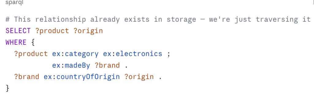
This is the architectural difference that matters. It’s not about syntax or query language preference. It’s about whether relationships are a key part of your data model or an afterthought recreated at runtime.
Think of it like a city’s road network. A relational database is like a city where roads don’t exist until you ask for directions – the GPS has to calculate every route from scratch every time. A knowledge graph is like a city where the roads are already built – you can just drive along them.
Challenge 1 – Simple Lookup
“Find all products made by Logitech”
Python/CSV:
import pandas as pd
df = pd.read_csv('products.csv')
logitech_products = df[df['brand'] == 'Logitech']
SQL:
SELECT name, price
FROM products
WHERE brand = 'Logitech'
ORDER BY price;
SPARQL:
SELECT ?name ?price
WHERE {
   ?product ex:madeBy ex:logitech ;
            ex:name ?name ;
            ex:price ?price .
}
Verdict: All three methods perform well. CSV filtering is likely the simplest option. If this is all you need to do with your data, a knowledge graph adds unnecessary complexity. This is an important point to consider. Knowledge graphs are not always superior. For simple lookups on flat data, they can be excessive.
Challenge 2 – Multi-Hop Relationships
“Find all products related to Logitech products, then find products related to those.”
This is where things begin to differ.
CSV Approach:
# Step 1: Find Logitech products
logitech_ids = df[df['brand'] == 'Logitech']['product_id'].tolist()

# Step 2: Find directly related products
related_ids = []
for pid in logitech_ids:
    row = df[df['product_id'] == pid]
    if not row['related_to'].isna().values[0]:
        related_ids.extend(row['related_to'].values[0].split('|'))

# Step 3: Find products related to those (second hop)
second_hop = []
for pid in related_ids:
    row = df[df['product_id'] == pid]
    if not row['related_to'].isna().values[0]:
        second_hop.extend(row['related_to'].values[0].split('|'))
# Already messy — and this is only 2 hops
This method requires manual traversal. Each hop means a new loop. The related_to column contains pipe-separated IDs as a string. It’s a flat structure trying to mimic a graph. It completely falls apart with three or more hops.
SQL Approach:
-- Two hops requires a self-join
SELECT DISTINCT p3.name
FROM products p1
JOIN products p2 ONFIND_IN_SET(p2.product_id, REPLACE(p1.related_to, '|', ','))
JOIN products p3 ON FIND_IN_SET(p3.product_id,REPLACE(p2.related_to, '|', ','))
WHERE p1.brand = 'Logitech'
This method is already tricky. For three hops, you need to add another join. For variable-depth traversal – “find everything connected to Logitech products at any depth” – you need a recursive CTE, which many databases can handle but it adds significant complexity.
WITH RECURSIVE related_products AS (
  -- Base case: direct Logitech products
  SELECT product_id, name, related_to,0 as depth FROM products WHERE brand =  'Logitech'
  UNION ALL
  -- Recursive case: products related to those
  SELECT p.product_id, p.name, p.related_to, rp.depth + 1 FROM products p
  JOIN related_products rp
    ON FIND_IN_SET(p.product_id, REPLACE(rp.related_to, '|', ','))
  WHERE rp.depth < 5  -- You have to arbitrarily limit depth
)
SELECT DISTINCT name FROM related_products;
You’re battling the data model. The relationships aren’t stored; they are reconstructed from strings, hop by hop, while facing an arbitrary depth limit because the database lacks a native way to handle graph traversal.
SPARQL with property paths:
SELECT DISTINCT ?relatedProduct ?name
WHERE {
  ?logitech_product ex:madeBy ex:logitech .
  ?logitech_productex:relatedTo+ ?relatedProduct .
  ?relatedProduct ex:name ?name .
}
The + operator means “one or more hops.” The graph automatically traverses the entire connected subgraph, no matter the depth, without needing you to specify how many hops to take. Relationships are stored physically; traversal is simply about following pointers.
Cypher equivalent:
MATCH (brand:Brand {name: "Logitech"})<-[:MADE_BY]-(p:Product)-[:RELATED_TO*1..]->(related:Product)
RETURN DISTINCT related.name
Verdict: CSV fails at 2 or more hops. SQL requires recursive CTEs with arbitrary depth limits. Both graph methods manage this easily with a single query. Here, the key distinction – stored connections vs. runtime reconstruction – creates a fundamentally different outcome.
Challenge 3 – Schema Evolution
“Add a new relationship type: frequently_bought_with”
Your product team wants to track which products are often bought together. This differs from related_to; it relies on purchase data instead of editorial choices.
CSV Approach:
Add a new column, frequently_bought_with. However, related_to is already a pipe-separated string of IDs, so you’re adding another one. Now you have two columns trying to show graph relationships in a flat format. What happens when you add a third relationship type? A fourth? The file becomes hard to manage, and the code to read it becomes unreliable.
SQL Approach:
-- Option 1: Add a new column
ALTER TABLE products ADD COLUMN frequently_bought_with VARCHAR(500);
-- Option 2: Create a junction table (better practice)
CREATE TABLE product_relationships (
product_id VARCHAR(10),
related_product_id VARCHAR(10),
relationship_type VARCHAR(50),
PRIMARY KEY (product_id, related_product_id, relationship_type)
);
The junction table is the right approach in SQL, but now you have created a manually maintained edge table. You’re trying to implement a graph in a relational database. Each new relationship type adds another value in the relationship_type column. Your queries become more complicated. Your schema documentation grows longer. Plus, you still lack native graph traversal.
Knowledge Graph:
Just add new triples – no schema change required
ex:p001 ex:frequently-bought-with ex:p003 .
ex:p002 ex:frequently-bought-with ex:p008 .
ex:p004 ex:frequently-bought-with ex:p005 .
Three lines. No migration script. No ALTER TABLE. No junction table. The graph naturally accepts new relationship types because relationships are first-class elements, not columns or rows in a junction. The schema is the ontology, which can be expanded without affecting existing data.
Verdict: SQL needs schema updates or increasingly complex junction tables. CSV becomes hard to manage. Knowledge graphs accommodate new relationship types without structural changes. In fields where relationships change often, which applies to most real-world scenarios, this flexibility adds up over time.
Challenge 4 – Inference
“Find all accessories compatible with Logitech products – including products never explicitly tagged as compatible but whose category and brand relationships imply compatibility”
There is no good solution for this in SQL or CSV. Let me explain.
In our dataset, we know:
- USB Hub (P003) is
related_toWireless Keyboard (P001) and Wireless Mouse (P002). - Laptop Stand (P008) is
related_toP001, P002, and P003. - Both P003 and P008 are in the Electronics category.
But we haven’t explicitly stated that anything compatible with a Wireless Keyboard is probably also compatible with a Wireless Mouse; that’s an inference. It logically follows from the data, but it was never recorded.
CSV/SQL Approach:
You cannot automatically derive this inference. You would need to manually find and store every compatibility relationship. As your catalog expands, this becomes unmanageable.
Knowledge Graph with OWL reasoning:
# Define in ontology: if X is compatible with Y and Y is related to Z, then X is likely compatible with Z (transitive compatibility)

ex:compatibleWith a owl:TransitiveProperty .


# Store what we know explicitly

ex:p003 ex:compatibleWith ex:p001 .
ex:p003 ex:compatibleWith ex:p002 .
# Query: find everything compatible with Logitech products
# The reasoner derives transitive compatibility automatically

SELECT ?accessory ?name
WHERE {
?logitech_product ex:madeBy ex:logitech .
?accessory ex:compatibleWith ?logitech_product ;
           ex:name ?name .
}
The OWL reasoner automatically derives the transitive closure; if A is compatible with B and B is compatible with C, then A is compatible with C, without you needing to store that fact explicitly. As you add new products and compatibility relationships, the inferred facts update automatically.
Verdict: Inference has no equivalent in relational or flat file data models. This is a unique capability of knowledge graphs. For recommendation engines, compatibility matrices, and any field where indirect relationships matter, this can be truly transformative.
Challenge 5 – Interoperability
“Enrich our product catalogue with external data – product descriptions from Wikidata, brand information from external registries”
CSV/SQL Approach:
Export your data, call external APIs, merge results, and re-import. Create a custom ETL pipeline. This can create a maintenance burden. You need to map the schema every time the external source changes.
Knowledge Graph with SPARQL federation:
PREFIX wd: http://www.wikidata.org/entity/

SELECT ?product ?name ?wikidataDescription ?brandCountry
WHERE {
  # Your local data
  ?product ex:name ?name ;
           ex:madeBy ?brand .

  # Wikidata — queried live, no import needed
  SERVICE https://query.wikidata.org/sparql {
    ?wikidataItem rdfs:label ?name .
    ?wikidataItem schema:description ?wikidataDescription .
  }
}
Since your data uses URIs that match with shared vocabularies, you can query both your local knowledge graph and public linked data sources at the same time. There is no need for import, ETL, or schema mapping. The shared URI space serves as the integration layer.
Verdict: Federated querying is a unique capability of RDF/SPARQL. For organizations that want to enhance internal data with external sources like Wikidata, DBpedia, or industry registries, this approach removes entire categories of data pipeline work.
When Should You NOT Use a Knowledge Graph?
The honest answer is often.
Knowledge graphs are not suitable when:
Your data is truly flat. If you are storing time series sensor readings, transaction logs, or simple inventory counts, there are no meaningful relationships to navigate. A relational database or even a CSV is simpler and faster.
Your team lacks graph experience. The learning curve for SPARQL, OWL, and RDF tools is significant. If your team is only familiar with SQL, the productivity cost of switching to graph technology may not be worth it for your specific case.
You need very high write throughput. Knowledge graph databases are optimized for workloads heavy on reading and navigating. If you are writing millions of records per second, a time-series database or columnar store is a better option.
Your relationships are simple and stable. If your data features two or three well-defined types of relationships that do not change, a relational database with a junction table works perfectly. You do not need a graph.
You are building a simple CRUD application. If your main tasks are creating, reading, updating, or deleting individual records without significant navigation needs, relational databases are faster to develop with and easier to manage.
The engineers who gain the most from knowledge graphs use them when the data model truly requires it, not as a default or just because it’s an interesting technology.
The Decision Point
Looking back at our five challenges, a pattern emerges:
| Challenge | CSV | SQL | Knowledge Graph |
| Simple lookup | |||
| Multi-hop traversal | Complex | ||
| Schema evolution | Migrations | ||
| Inference | |||
| Interoperability |
The crossover point, where a knowledge graph becomes worthwhile, is when your data has multiple evolving relationship types. It is also when you need to traverse those relationships at different depths or derive facts that aren’t explicitly stored.
For e-commerce: product catalogs, recommendation engines, supplier networks, and customer journey graphs all belong in knowledge graph territory. Simple inventory management and order processing do not.
What’s Next
Now that you know when a knowledge graph is the right choice, the next article will be hands-on. We will take this exact e-commerce dataset, convert it to RDF with Python, load it into a triple store, and run the SPARQL queries we’ve discussed. We will also do the same with Neo4j, so you can see both approaches working on real data.
If you’re just getting started, read “What is a Knowledge Graph?” first. If you want to understand the RDF versus property graph choice before diving into the tutorial, that comparison is here.